
In the previous parts of this Excel tutorial, you have been working on a spreadsheet that now looks like this:

To get the weekly cost of each chocolate bar, we need to multiply the Number of bars eaten in one week by the Price. This can then go in the Cost column. The standard way to multiply things is like this:
12 x 10 = 120
The "x" means multiply. In a spreadsheet, however, the letter "x" is not used to multiply things. Spreadsheets use the asterisk symbol instead (the one above the number 8 on your keyboard, in the UK). The previous sum would then look like this:
12 * 10 = 120
Actually, in Excel, you don't need much more than that to multiply. The only other thing you need is an equals sign before the formula. So to get the answer 120, you'd just enter this into any cell:
= 12 * 10
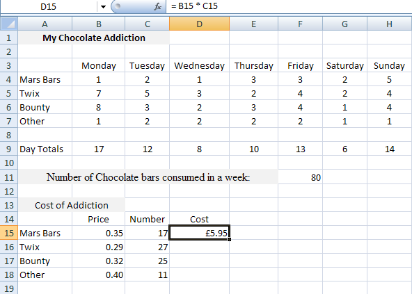
Instead of entering numbers directly, though, we'll enter a cell reference instead. To multiply, then, try this:
- Click into cell D15 on your spreadsheet, just below your Cost heading
- Now click into the Formula Bar at the top of Excel
- Type the following formula:
= B15 * C15
- Hit the enter key on your keyboard, and you should get an answer of 5.95
- Your spreadsheet will look like this (we've formatted the cell as a currency):
So to multiply in Excel , you do this:
= Cell Reference * Cell Reference
You type the equals sign first ( = ), followed by the first cell. Type an asterisk ( * ), and then the second cell. Hit the enter key, and Excel will multiply the two cells for you:
= B15 * C15
Once you have that first formula in place, you can use AutoFill for the others:

After you're done, you should have the same figures that we have in the Cost column.
In the next part of the tutorial, you'll complete this Excel spreadsheet by adding a weekly cost and a yearly cost.